Spiral Point

After today’s very generous mentions in Vasari Talk 22, I thought I’d better finish up another post. This builds on last week’s layout, with a twist!

It’s very easy to use Dynamo to build ‘dumb’ models, by just placing points at exact coordinates. But I’m intrigued by ways of using Dynamo to build proper parametric Revit components: Placing lots of points quickly to generate complex form, while at the same time relating those points together is useful ways. Last week’s post was a first step on that path, and this post takes it a bit further.

So, last week’s post ended by using a ‘Reference Point on Edge’ node to host a point on a curve. This layout hosts a point on that point’s YZ reference plane, so that as the first point moves, the second point is carried along:

You’ll recognise the arrangement of nodes at the top of the layout from the last post: A pair of reference points connected by a curve (aka straight line), and then a reference point hosted on that curve. The parametric position of the hosted point along the curve is driven by a slider node, and the slider is set to give values between 0 and 1: By moving the slider, the hosted point moves from one end of the curve to the other.

This hosted reference point is fed to a new User node ‘GetCoordinatePlaneReferenceYZ’, which gets the point’s YZ reference plane. The refplane is fed into the ‘face’ input of a ‘Reference Pont on Face’ node, which places a point on the plane. I was surprised that the face input would accept a reference rather than a face, but it’s great that it does.

Now that would be fine, because the plane-hosted point would move with the curve-hosted one, but I was inspired by David Light’s 2010 video of a helical adaptive component to try and make the point move in a helix or spiral, and the set of nodes at the bottom of the layout make that happen.

Helical movement is a combination of moving around in a circle and moving along a line. The slider makes the points move along the line, so I just had to get the plane-hosted point to move in a circle on the plane.

The slider feeds into a multiply node along with the value 2π, and so by moving the slider from 0 to 1, the multiply produces an angle value from 0 to 2π radians. The angle is fed into Sine and Cosine nodes to give Y and Z coordinates, multiplied by the number 20 at the bottom to give a 20 unit radius circle.

The only new User node required was GetCoordinateReferencePlaneYZ, which wraps a snippet of Python that makes the API call:

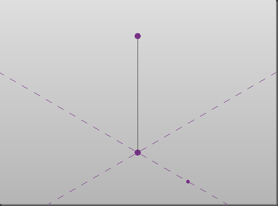
When run, you get a simple line and two hosted points:

When run automatically, you get to slide the line-hosted point up and down the line, while the plane-hosted point moves in a spiral around it:

It’s just unfortunate that the slider is so small on screen that it makes the movement a bit jerky. But I think the video just about shows the idea.

And here’s the source: Spiral Point

Curve By Points and Reference Point On Edge

Post-pumpkin, I’ve been exploring the conceptual massing environment in more depth, both through the user interface and via the API. So I thought it would be fun to implement the WikiHelp API examples in Dynamo. This is the first, and follows this WkiHelp example:

The left hand side is not very interesting: Just some hard-coded XYZs, fed into a List node. The list of XYZs is then fed to a Reference Point node to generate a list of reference points (the Reference Point node is one of the few that will equally accept either a single value or a list). And then the refpoints are fed into a Curve By Points node to generate the curve.

The last two nodes generate the hosted point on the curve (described in the WikiHelp text but currently missing from the code listing). The Reference Point On Edge node creates the point and the Number node sets the parametric position of the hosted point along the curve. Replacing the Number node with a slider allows you to move the point along the curve dynamically (with Run Automatically on, and a reasonably fast computer).

And here’s the source: WH 14-1 Curve By Points

Punkinator Dissection

This is a description of how my Dynamo-powered Punkinator works. I’ll start with an overall, top-down description, and then move on to a bottom-up explanation of each of the nodes.

The pumpkin is a loft form generated from a set of profiles. Each profile is a loop of model lines drawn on a horizontal plane, and the loops get smaller towards the top and bottom of the form to produce the generally spherical shape. You can see the purple reference points used to create the loops in this screenshot of a pumpkin in X-Ray View (you can’t see the model lines because the refpoints are so closely spaced):

The reference points are calculated using Johan Gielis’ superformula of an ellipse, equation (2) in his 2003 paper:

This looks a bit intimidating, but the aim of it is to calculate a radius (r) from an angle, phi (Φ). Then use the radius and angle as polar coordinates to plot a point. If you plot a series of points using different input angles, you can join the dots to create a loop.

Why use the superformula? Well the sample plots in Gielis’ paper suggested that it could create some nice organic shapes, given the right input parameters a, b, m, n₁, n₂ and n₃. And there are several images online that show pumpkin-like superformula shapes.

So I figured that if I could generate a series of pumpkin-shaped loops using the superformula, I could loft a form through them and create a pumpkin for Zach Kron’s 4th Annual Parametric Pumpkin Carving. And it worked!

Now on to the more detailed explanation, starting at the bottom:

Superformula

This is the fundamental node. It calculates the radius from a given angle, based on the superformula with input parameters a, b, m, n₁, n₂ and n₃.

It is a fairly straightforward implementation of the superformula. The angle, m, a, and b inputs are at the left; the n1, n2 and n3 inputs are in the middle. The rest is just the mathematical manipulation.

The Superformula node makes use of a couple of helper nodes: Abs, which calculates the absolute value of the input:

and x^y which calculates x to the power y using a snippet of Python:

This is the only bit of Python in the solution. I guess you could make a recursive pure-Dynamo node that would calculate a power. But at the time, the Python implementation was more direct.

Incidentally, this also shows one way of pushing multiple inputs into a Python node: The List node packages the two input values into one list; and then the Python code unpacks the list elements into individual variables.

I put the Transaction node in because while I was testing, Dynamo complained that it needed one. I don’t really see why it should need one at this point, so I may try taking it out again now.

Superformula XYZ

This creates a Revit API XYZ element using the distance and angle from the superformula node:

It also has a scale input, to scale the loop up and down, and a z input, to move the loop to different z values.

Superformula XYZ uses just one helper node, Polar XYZ:

This uses a bit of trigonometry to calculate the X and Y values from the input polar coordinate, and then calls the standard XYZ node.

Why do I keep creating these helper nodes? Three reasons:

1. You can test and debug the helper node in isolation
2. It makes the main node simpler to understand
3. You can re-use the helper nodes in other solutions

Superformula Loop

This creates a loop of reference points from the superformula, and then connects them with lines:

The nodes at the bottom of the layout divide a full circle into a sequence of angles. The Number node on the left is where you set the number of divisions (i.e. the number of points in the loop). Higher numbers create smoother loops, more slowly.

The upper Map node calls Superformula XYZ once for each angle, and then the Reference Point node and ConnectPoints nodes generate the loop of points and lines. ConnectPoints is a user node that ships with Dynamo.

Superformula Loop uses two helper nodes: 2pi/n, which gives the angle that is 1/nth of a circle:

Dynamo measures angles in radians, and there are 2π radians in a circle (don’t be put off by the radians: They’re just a different way of measuring angles, like degrees but more convenient for some maths).

…And ‘Build Sequence 0 to n’, which builds an integer sequence from 0 to n:

The standard Build Sequence node excludes the end value, and if I used this to generate my loop, it would leave a gap. I need to generate a complete sequence of angles from 0 up to and including 2π. Hence the custom node.

Superformula Loop Driver 2

This calculates the z-value and scale for an individual loop:

So I wanted the pumpkin to be roughly spherical, which meant that I needed to generate a series of circularish/pumpkin-shaped loops positioned and scaled like lines of latitude on the earth. So  I’m using polar coordinates in a vertical plane to generate the z and scale values for Superformula Loop.

Why didn’t I just include this calculation inside Superformula Loop? Three reasons (similar to the reasons for helper nodes):

1. Each node just does one thing: You can test and debug it in isolation
2. Each node is simpler, and easier to understand
3. I might want to re-use either the Loop node or the Driver node (tweaked) in other solutions.

Why is it called Superformula Loop Driver 2? Because Superformula Loop Driver 1 didn’t work.

Punkinator

This is the main layout:

The bottom part of the layout generates a sequence of angles (in the vertical plane) to position the loops vertically. Half a circle (180 degrees) is π radians, so I space the top and bottom loops 0.1 radians off vertical, and then divide the remaining vertical angle by the bottom-left Number input to generate the loops.

The top part of the layout has the parameter input nodes for the superformula (which is driven by the Map), and then over on the right-hand side, there is the Loft Form node, which actually creates the form. the two Watch nodes are just debugging aids, so I can see the list of loops in the top Watch, and the list of angles in the bottom one.

Whew! That’s all there is to it.

Just a couple of caveats: The code runs slowly. If you want to try it out, I’d start by putting a small number like 4 or 8 into the bottom-left number node in Superformula Loop because that will make it complete faster. I’d restart Dynamo if you want to change this number again, because it will probably break the loft if you change it on the fly. The code only runs with the debug switch on. As Zach found, it only runs in Revit, not in Vasari (not sure why not just yet). If you try it, thank you, and do let me know how you get on!

And here’s the source.

Revitator’s Punkinator

A week ago today I was determinedly hacking away at Dynamo, intent on creating a pumpkin, any kind of pumpkin, for Zach Kron’s 4th Annual Parametric Pumpkin Carving. My first two attempts at pumpkin-carving had merely revealed my lack of skill with nested profiles and adaptive components, and time was running out.

So I fell back on an approach I’d used previously (in particular for the twisting tower I presented at Manchester Revit User Group (MRUG) back in September): Build a loft from a series of loops.

Now Dynamo, being Alpha code, can be a bit tricky, and I didn’t get the thing running at all until midnight. And then it ran glacially slow. But it did create pumpkins; or pumpkin-like things; or (depending on the parameters), totally un-pumpkin-like things. So I snapped a couple of screenshots, zipped the files up, wrote a quick explanation, and sent the whole lot off to Zach. And then went to bed thinking, ‘Well, at least I made something this year.’

And then, surprise, delight, my pumpkin won Mostest Parametric!

Just goes to show: Put the effort in and turn up to the event, you might just be lucky!

DesignScript - Points

Autodesk Labs have just released DesignScript as a Technology Preview, so I’ve been looking at porting some of Nathan Miller’s Proving Ground RevitPythonScript examples, just to see how DesignScript works. This first post summarises the Point Creation examples:

Single Point

This is the simplest example: Create a point at specified coordinates.

import("ProtoGeometry.dll");
// create a point with x, y, and z coordinates
x_pos = 10;
y_pos = 10;
z_pos = 0;
pCoord = Point.ByCoordinates(x_pos, y_pos, z_pos);

This was adapted from the example on page 17 of the DesignScript Language Manual, version 09. It is very simple: Import the ProtoGeometry dll, define the coordinates and call Point.ByCoordinates(x,y,z).

Row of Points

Create a row of points at specified xy values:

import("ProtoGeometry.dll");
// create a row of points
x_pos = 0..100..10;
y_pos = 0..100..10;
z_pos = 0;
pCoord = Point.ByCoordinates(x_pos, y_pos, z_pos);

This example is hardly more complex. Just by defining the x and y coordinates as ranges rather than single values, Point.ByCoordinates generates a row of points.

Grid of Points

Create a grid of points:

import("ProtoGeometry.dll");
// create a grid of points
x_pos = 0..100..10;
y_pos = 0..100..10;
z_pos = 0;
pCoord = Point.ByCoordinates(x_pos<1>, y_pos<2>, z_pos);

And just by making a tiny change to the code, adding the Replication Guides <1> and <2> to the Point.ByCoordinates call, Point.ByCoordinates generates a grid of points.

Sine Wave Points

Create a grid of points, where the z-value of each point is a function of the x and y coordinates.

import("ProtoGeometry.dll");
import("Math.dll");
def RadiansToDegrees(n)
{
    return = n * 360/(2 * 3.142);
}
def CosXPlusSinY(x, y)
{
    return = Math.Cos(RadiansToDegrees(x)) + Math.Sin(RadiansToDegrees(y));
}
def PointZ(x, y)
{
    z = CosXPlusSinY(x, y);
    s = Print(z);
    return = Point.ByCoordinates(10 * x, 10 * y, 10 * z);
}
// create a grid of points where z = f(xy) 
x_pos = 0..30;
y_pos = 0..30;
pCoord = PointZ(x_pos<1>, y_pos<2>);

Now this is suddenly much more complex. The simple range and replication guide tricks work for simple cases, but are harder to apply in more real-world examples.

I wanted to use the replication guides to generate the grid (I could have fallen back on nested loops, of course, but that would be a shame). There doesn’t seem to be a way to include the z function inline, like this:

pcoord = Point.ByCoordinate(x_pos<1>, y_pos<2>,CosXPlusSinY(x_pos,y_pos))   //fail

So I wrapped the z-calculation and the Point.ByCoordinates call in a custom function, PointZ(x,y). In this way, I could use the replication guides in the call to PointZ, and

The other slight complexity is that both Python and Dynamo use radian values for their trig functions, DesignScript expects degrees. Hence the RadiansToDegrees function (with a dodgy value for pi because, well, I haven’t been able to find the correct syntax for DesignScript’s PI() function).

And here’s the source: DesignScript Points examples.

Dynamo - Indexed Family Instances

Once classic way to create forms in Revit is to place multiple family instances that are driven by an indexed instance parameter. Zach Kron gives a good explanation in his post Parametric Patterns VI: Increment. The only tedium is in placing and indexing all the instances.

I wondered how hard it would be to place and index the instances using Dynamo, and this is the result:

The Family Type Selector and the Instance Parameter Selector allow you to choose the family type to place and the driving parameter. The Build Sequence node and its inputs generate the sequence of values for the driving parameter.

The Map node calls my user node ‘Family Instance Creator – Indexed’ once for each number in the sequence, and each time, the node creates a family instance and sets the driving parameter:

This is fairly straightforward. All the instances are placed at 0,0,0. The Family Instance Creator node creates the instance, and the Set Instance Parameter node sets the driving parameter.

And here is the result, using a simple twisting box family:

Finally, here is the source: Indexed Family Instances.

Dynamo - Plane using 3 Points

This is the second method of creating a Plane shown by Nathan Miller, ported into Revit Dynamo:

Again, it’s fairly simple. The only tricky bit is that Dynamo doesn’t expose the Revit API call NewPlane(CurveArray), so I’ve made a Python-based user node to wrap that functionality.

The three points in this example are made with my XYZ… user nodes, and fed into the pair of Line nodes to create two geometry lines. Note the order of the points: The end of one line has to connect to the start of the next. The List node puts the two lines into a list to feed into the Plane by Curves user node. Again, the Transaction node is there because Dynamo asked for it, and the Watch is there so you can see that something happens.

The Plane by Curves user node is simply a wrapper for a bit of Python:

Here is the Python script:

The input from Dynamo is a list of curves or lines. But you cannot use that list of curves as input to NewPlane. You have to unpack the list and put the curves into a Revit API CurveArray object, because that is the type of input that NewPlane(CurveArray) expects. So the “carray =…” line creates the empty CurveArray, and the “for i in range…” lines append each curve to the CurveArray.

This shows the power of the Python node for extending Dynamo. The NewPlane(CurveArray) call isn’t exposed in base Dynamo, but it is fairly easy to add with a Python-based user node. I’m no Python expert (and this node owes a lot to Nathan Miller’s original RevitPythonShell script), but it didn’t take too much trial-and-error to get it working.

And here’s the source: Link to Dynamo Definition PG 2.2 Sketch Plane 3 Points.

Dynamo - Plane using World XYZ

Nathan Miller has two examples of creating Planes in RevitPythonShell. This is the first, ported into Revit Dynamo:

It is very simple. I figured that I’d be using XYZ.BasisZ and XYZ.Zero a fair bit, so it made sense to implement them as User Nodes. These are fed into the Plane node, which is in turn fed into the Sketch Plane node.

The Transaction node wraps the whole thing in a Revit Transaction. At the moment, I add a Transaction node when Dynamo complains that it needs one. Seems to be working so far.

The Watch node just allows you to see that something has happened when you run the code.

Of the two User Nodes, here is XYZ.BasisZ:

And here is XYZ.Zero:

As you can see, both User Nodes wrap a snippet of Python that calls the Revit API. I’ve found that you need to give the Python Script node an input to make it work, hence the otherwise superfluous Number nodes. Not sure if there’s a way to fix that just now.

And here’s the source: Link to Dynamo Definition PG 2.1 Sketch Plane World XYZ.dyn. Again, it’s a zip containing the dyn file and the two User Node dyf files. Open the dyfs first to load them into Dynamo’s library.

Dynamo - Sine Wave Points

Last Dynamo ‘Create Points’ example, porting ‘Sine Wave Points’ from Nathan Miller’s Proving Ground Wiki, Create Points page.

This is the trickiest example so far. The two Build Sequence nodes at bottom left create the X and Y values. The Cartesian Product node applies the function ‘comb’ to each pair of XY values. I’ve created the function as a couple of User Nodes, and then Mapped the output into the XYZ Scale node to scale the grid up by 10x.

As an aside, note the difference between Cartesian Product and Combine nodes. Cartesian gives {X₁Y₁, X₁Y₂, X₁Y₃, … X₂Y₁, X₂Y₂, … X_nY_n} which makes a grid; while Combine gives {X₁Y₁, X₂Y₂, X₃Y₃, … X_nY_n} which would just make a line. More info: Cartesian Product on Wikipedia.

Regarding the User Nodes: I tend to use them to wrap custom code for easy testing. If you build a big plate of spaghetti, it’s very hard to tell what’s not working properly. If you break the code into ‘User Node’ chunks, you can test each piece in isolation to make sure it works. Also, with the Map-like nodes, I prefer to feed them a User Node function because it’s clear how the inputs are going to be mapped. I’m not even sure some of my Mapped functions could be made without User Nodes.

Anyhow, this example uses two User Nodes. First up is cos(x)+sin(y):

Which very obviously does what it says on the tin.

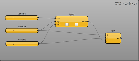
Next is XYZ - z=f(xy), which I’m quietly pleased with:

This uses the input function f to generate a z value from the input x and y values, and then outputs an XYZ object. I wasn’t sure whether you could pass a function into a User Node like this. It’s great that you can, since it makes the initial layout much more flexible: Just substitute a different function in place of cos(x)+sin(y) to generate a different set of z values for the grid.

I’ve used an Apply here rather than a Combine, since the node will only accept one pair of xy values at a time. If you wanted a node that would accept list inputs, you’d also need to Combine the XYZ. I’ll post an example when I find an application.

Here’s the source: Dynamo Definition PG 1.4c Sine Wave Points.zip. The zip file contains both the .dyn file and the two User Node .dyf files. Open each of the .dyf files in turn to load them into Dynamo’s library, and then open the .dyn.

Dynamo - Grid of Points

Third in the series of basic Dynamo examples. This time following Nathan Miller’s RevitPythonShell ‘Grid of Points’ example, from the Proving Ground Wiki, Create Points page.

This example is really easy because Dynamo has a built-in XYZ Grid node. You just feed the relevant parameters into the node, and route the resulting list of XYZ objects to a Reference Point node to generate the grid of points.

Link to Dynamo Definition PG 1.3 Reference Point Grid.zip

Incidentally, to make any of these simple examples work in Dynamo, just use the Open… command from the File menu to open the .dyn file. It will open into the Home workspace, and you can Run it from there.

Dynamo – Row of Points

This is a Dynamo re-working of Nathan Miller’s RevitPythonShell ‘Row of Points’ example, from the Proving Ground Wiki, Create Points page

At the bottom left, the Build Sequence node is the equivalent of Nathan’s for-next loop. It generates a sequence (or list) of integers from 0 to 9. The two Map nodes create the X and Y values, and the Combine calls the XYZ node for each pair of X and Y values.
You can see that the program structure is quite different to a conventional, linear language like Python, C or Basic. The list-processing is like Lisp, of course, but the way the data flows between nodes takes a bit of getting used to.
For example, the Map node has two inputs: f(x) which is a function, and seq which is a sequence or list. The Map node applies the function to each item in the sequence, and outputs the results as a new sequence. In this case, I’ve used the function X (multiply). I’ve fed the value 10 into the multiply node’s x input, and left the y input for the Map node to use.
In the same way, my Combine node takes a function (comb) and two sequences (list1 and list2)as inputs . It applies the function to the two sequences, and outputs the results as a new sequence.
Link to Dynamo Definition PG 1.1 Reference Point.dyn

Dynamo – Single Point

This is a Dynamo re-working of Nathan Miller’s RevitPythonShell ‘Single Point’ example, from the Proving Ground Wiki, Create Points page.

I’m using the three Number Sliders to generate the X, Y and Z coordinates. The XYZ Node creates a behind-the-scenes Revit XYZ object, and the the Reference Point creates the visible Revit Reference Point object.
If you select Run Automatically in Dynamo, then the Reference Point in Revit will move as you adjust the Number Sliders in Dynamo.
Link to Dynamo Definition PG 1.1 Reference Point.dyn

Where to get Dynamo - Video

An extract from my presentation to Manchester Revit User Group, showing where to get Dynamo for Vasari and Revit, and how to get started. Another test. Sound quality is terrible.




Link to video on Screencast

MRUG Presentation

Last week I presented Revit Dynamo to Manchester Revit User Group. I’ve uploaded the (four) slides to Slideshare:

MRUG Presentation - Revit Dynamo from revitator

There were only four slides because most of the presentation consisted of live demonstration and pointers to further information on the web.
(To an extent, this post is a test to see how Slideshare works. So far it's not looking great, because the slides are not showing up reliably. I'll have another look later and see whether it is conversion lag)
Edit: No, still not showing up in the browser. Shows fine on Slideshare site. Shows fine in Blogger editing window. Perplexed.